RL-ACD

Read the paper

ACD Context

• ACD: approximate a dense mesh with a few convex pieces (collisions for games/VR/robotics sim). Objectives: 1) minimize # of components $|M|$, 2) minimize total concavity ${\sum }_{m_i\in M}\text{Concavity}(m_i)$
• Prior methods: concavity metric + plane-selection strategy. Greedy (V-HACD, NavACD) is fast but leaves redundant pieces. CoACD uses MCTS over plane cuts which is better, but simulates many exact cuts per step which is slow
• RL-ACD: learning a policy that predicts the cutting plane

Pipeline

• State = current set of pieces $M=\{m_i\}$. Action = $⟨i,p⟩$ (which piece & plane, $p\in {\mathbb{R}}^4$), transition = boolean cut: $M^{\prime }=M\cup \{m_i^l,m_i^r\}-\{m_i\}$
• Reward $r_1=\frac{|CH(m_i)|-|CH(m_i^l)|-|CH(m_i^r)|}{|CH(m)|}$ (hull volume removed normalized by the whole mesh) + a completion bonus at the end so it stops cutting
• Policy only sees $m_i$, never $M$ (POMDP obs $O(M,i)=m_i$). This is fine because reward adds across pieces so other pieces don’t change the best cut for $m_i$
• State encoder: sample 2048 points on $m_i$ and on $CH(m_i)$, normalize, run through frozen pre-trained I2P-MAE $\to s(m_i)=(F(m_i),F(CH(m_i)))$
• Discrete action space, fixed candidate set $P(m_i)$ with choices (a) equidistant axis-aligned XYZ planes (b) PCA-axis-aligned planes (c) concave-edge planes
• Same $|P|$ for every piece, pieces are normalized before encoding so every piece has the same $K$ candidates. DQN: $K$ output heads, head $j$ = $Q(p_j,m_i)$. Only encode once, one MLP pass, argmax
• Deploy: whole mesh starts as one piece. In each step encode every piece, one MLP pass each, take the global best $⟨i,p⟩$ and perform that cut, repeat until every piece’s concavity < threshold. This is greedy but over a quantity that accounts for the future, $Q$, instead of immediate concavity reduction like priors
• Q-net is a small 4-layer MLP $\{1024,512,256,128\}$ with $s(m_i)$ in, $K$ Q-values out. Soft Q-learning (soft-max instead of max in the Bellman target)

Baseline

V-HACD, NavACD (greedy) + CoACD (MCTS)

Results

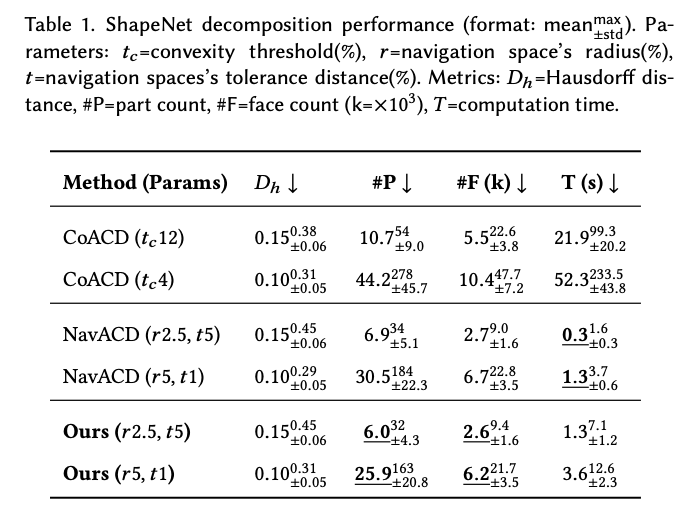Table 1. ShapeNet decomposition performance (format: meanmax ±std). Parameters: 𝑡𝑐=convexity threshold(%), 𝑟=navigation space’s radius(%), 𝑡=navigation spaces’s tolerance distance(%). Metrics: 𝐷ℎ=Hausdorff distance, #P=part count, #F=face count (k=×103 ), 𝑇 =computation time

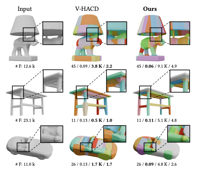Fig. 6. Comparison with V-HACD using the same number of decomposed parts. Numbers below each result indicate the number of convex parts, Hausdorff distance, face number, and decomposition time (𝑠). Close-up views highlight decomposition quality.

Dual-state Bellman loss

We don’t use standard Q-learning because

• $Q(s,a)=r+\gamma {\max }_{a^{\prime }}Q(s^{\prime },a^{\prime })$ yields exactly one next state $s^{\prime }$ when we should have two (two children from slice)
• The true $s^{\prime }$ = all of $M^{\prime }$ which we do not want to encode

RL-ACD

• Assume value of a pile of pieces = sum of each piece’s value, $V(M)={\sum }_{i}V(m_i)$. Cutting $m_i$ doesn’t touch the others, so they cancel out of the target. Therefore we can have the network look at one piece at a time
• Score of a piece = score of its best available cut, $V(m_i)={\max }_{p}Q(p,m_i)$
• Dual-state Bellman loss: $\mathbb{E}\Vert r+{\gamma }^{l}V(m_i^l)+{\gamma }^{r}V(m_i^r)-Q(p,m_i){\Vert }^2$
• ${\gamma }^l=|CH(m_i^l)|/|CH(m_i)|$, ${\gamma }^r$ same. This weights bigger (by volume) halves more
• Halves don’t overlap so ${\gamma }^l+{\gamma }^r\le 1$, which is the contraction condition $⟹$ converges. and trains faster than one shared $\gamma$
• Everything else is deep soft Q-learning

Learned policy vs. tree search

MCTS

• Every step simulates exact cuts (slice mesh, hull children) for many candidate planes over multiple lookahead steps to find the best cut
• Cost = # candidates * depth * exact-cut
• Nothing carries over between meshes

RL policy

• Exact cuts happen during training and get stored in a replay buffer. At runtime, one point cloud gets encoded + one MLP pass per piece, then best cut is chosen using Q-values, one exact cut executed
• A bigger candidate plane set is free, just more MLP outputs
• The Q value already accounts for the lookahead since the Bellman target folds in the future value of the two children, instead of simulating